FlashQLA: CP-/Bwd-Friendly Fused Linear Attention Kernels for GDN
文章目录
Introduction#
Following the release of Qwen3-Next, Gated Delta Network (GDN) has become the workhorse attention layer across the Qwen family — from Qwen3-Next-80B-A3B all the way to the subsequent Qwen3.5 / Qwen3.6 series. As models scale to 397A17B / 122A10B / 35B / 27B and context windows stretch beyond 256K, the overhead of the GDN block in end-to-end training and inference has become non-negligible.
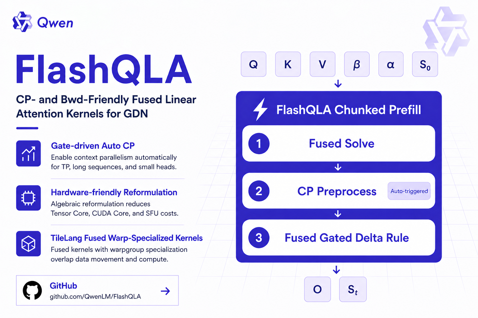
Today we officially open-source FlashQLA: a high-performance linear attention kernel library built on TileLang. FlashQLA applies reasonable operator fusion and performance optimization to the forward and backward passes of GDN Chunked Prefill, achieving 2-3× forward speedup and 2× backward speedup over the FLA Triton kernel across multiple scenarios on NVIDIA Hopper. The efficiency gains are particularly pronounced in pretraining scenarios and edge-side agentic inference.
Key highlights of this release:
Gate-driven automatic intra-card context parallelism. By exploiting the exponential decay property of the GDN gate, FlashQLA automatically enables intra-card CP under TP, long-sequence, and small-head-count settings, improving GPU SM utilization.
Hardware-friendly algebraic reformulation. We reformulate the forward and backward flows of GDN Chunked Prefill to a certain extent, effectively reducing Tensor Core, CUDA Core, and SFU overhead without sacrificing numerical precision.
TileLang fused warp-specialized kernels. Rather than following the step-by-step decomposition into independent kernels, nor fusing the entire computation flow into a single kernel, we take CP and backward requirements into account, use TileLang to build several key fused kernels, and manually implement warpgroup specialization to overlap data movement, Tensor Core computation, and CUDA Core computation.
FlashQLA code and benchmarks are open-sourced at github.com/QwenLM/FlashQLA.
Key Problems in FLA GDN Chunked Prefill#
Let us first review the forward computation flow of GDN Chunked Prefill, taking chunk index $i$ as an example:
- $A_i \gets \left(I+\mathrm{StrictLower}\left( \mathrm{diag}(\beta_i)(\Gamma_i \odot K_iK_i^\intercal) \right)\right)^{-1}$
- $\left\{\begin{aligned} W_i &\gets A_i\mathrm{diag}(\beta_i)\mathrm{diag}(\gamma_i)K_i \\ U_i &\gets A_i\mathrm{diag}(\beta_i)V_i \end{aligned}\right.$
- $\left\{\begin{aligned} V_i’ &\gets U_i-W_iS_i \\ S_{i+1} &\gets \gamma_{i,C-1}S_i + K_i^\intercal\mathrm{diag}\left(\frac{\gamma_{i,C-1}}{\gamma_i}\right)V_i’ \end{aligned}\right.$
- $O_i \gets \mathrm{diag}({\gamma})Q_iS_i + \left(\mathrm{Lower}(\Gamma_i) \odot Q_iK_i^\intercal\right)V_i'$
Ignoring gate preprocessing and CP, each step of this flow corresponds to one kernel in FLA. This flow has two main efficiency problems:
- Most of the above are memory-bound kernels. The flow repeatedly reads $K$, $V$ and other data, while $W$, $U$, $S$ as intermediate variables must be written to HBM and then read by the next kernel, incurring significant memory access overhead.
- The recurrent nature of the SSM state means that the corresponding third step
chunk_gated_delta_rule_fwd_kernelcan only launchbatch_size * num_headsthread blocks simultaneously, resulting in low GPU utilization in small-model, small-batch, or TP scenarios.
The solutions to these two problems are contradictory. For the first problem, the most intuitive solution is to write a fully-fused kernel, where all data is accessed only once and all intermediate variables are kept on-chip. When batch_size * num_heads is large enough, this is certainly optimal. However, such a solution obviously runs into the second problem: for edge-side inference with small models and batch_size=1, or for large-model online deployments with TP where long-sequence inputs from coding agents etc. cannot launch a large enough batch for chunked prefill, the speedup of a fully-fused kernel over the original FLA implementation is limited.
The earliest solution to the second problem comes from how DeltaNet does context parallelism, which splits a long sequence into multiple sub-sequences, uses $S_0=0$ to parallelize the recurrence, and then computes an additional $M$ matrix to correct the recurrent results. This scheme was later optimized to insert a step before the recurrence kernel to compute the $S_0$ of each sub-sequence, and has now been merged into the FLA repository. For CP rank $j$, the specific preprocessing flow is:
- $\left\{\begin{aligned} S^\ast_{j,i+1} &\gets \gamma_{j,i,C-1}S^\ast_{j,i} + K_{j,i}^\intercal \mathrm{diag}\left(\frac{\gamma_{j,i,C-1}}{\gamma_{j,i}}\right) V’_{j,i} \\ M_{j,i+1} &\gets \left( \gamma_{j,i,C-1} I -K_{j,i}^\intercal \mathrm{diag}\left(\frac{\gamma_{j,i,C-1}}{\gamma_{j,i}}\right) W_{j,i} \right) M_{j,i} \end{aligned}\right.$
- $S_{j,0} \gets S^\ast_{j,0} + M_{j,0}S_{j-1,0}$
However, this CP scheme also has its drawbacks: first, it introduces significant extra computation, with the time complexity of recurrently computing the $M$ matrix even exceeding that of the $S$ matrix; second, it does not work well with fully-fused kernels, because matrix inversion and other steps must be performed before the $S_0$ of each sub-sequence can be computed.
A Balanced Solution: Fusing Kernels While Enabling Intra-Card CP#
Based on the two problems above, a compromise solution can be derived: split the GDN Chunked Prefill forward computation into two fused kernels, inserting CP-related preprocessing steps between them. After some transformations and simplifications, the following computation flow is obtained:
- $A_i \gets \left(I+\mathrm{StrictLower}\left( \mathrm{diag}(\beta_i)K_iK_i^\intercal\right)\right)^{-1}$
- CP Preprocess
- 2.1. $\left\{\begin{aligned} X_{j,i} &\gets -\beta_{j,i} A_{j,i}’^\intercal K_{j,i} \\ Y_{j,i} &\gets \gamma_{j,i,C-1} K_{j,i} S^\ast_{j,i} - \mathrm{diag}\left(\frac{\gamma_{j,i,C-1}}{\gamma_{j,i}}\right) V_{j,i} \\ Z_{j,i} &\gets K_{j,i} M_{j,i} \\ S^\ast_{j,i+1} &\gets \gamma_{j,i,C-1}S^\ast_{j,i} + X_{j,i}^\intercal Y_{j,i} \\ M_{j,i+1} &\gets \gamma_{j,i,C-1} \left( M_{j,i} + X_{j,i}^\intercal Z_{j,i} \right) \end{aligned}\right.$
- 2.2. $S_{j,0} \gets S^\ast_{j,0} + M_{j,0}S_{j-1,0}$
- $\left\{\begin{aligned} V_i^\Delta &\gets V_i - \mathrm{diag}(\gamma_i)K_iS_i \\ V_i’ &\gets \left(\Gamma_i \odot A_i\right)\mathrm{diag}(\beta_i)V_i^\Delta \\ S_{i+1} &\gets \gamma_{i,C-1}S_i + K_i^\intercal\mathrm{diag}\left(\frac{\gamma_{i,C-1}}{\gamma_i}\right)V_i’ \\ O_i &\gets \mathrm{diag}({\gamma_i})Q_iS_i + \left(\mathrm{Lower}(\Gamma_i) \odot Q_iK_i^\intercal\right)V_i’ \end{aligned}\right.$
We also designed a simple mathematical model to automatically determine the degree of parallelism. Let $N$ be the number of chunks in a sequence and $L$ be the number of chunks per CP rank. It is easy to see that the runtime of steps 2.1 and 3 is proportional to $L$, while the runtime of step 2.2 is proportional to $\frac NL$; therefore we can choose $L=\lambda \sqrt N$ to minimize total time, where $\lambda$ is a coefficient composed of batch_size, num_heads, and other hyperparameters.
In production, intra-card CP is not always needed. Following the original FLA implementation, step 3 can also increase parallelism by 2-4× via splitting v_head_dim, at the cost of redundant memory access to Q and K. Based on measured data, we enable CP only when batch_size * num_heads <= 40 or batch_size * num_heads <= 56 && seq_len >= 8192.
Further Optimization via Gate Decay#
Revisiting the GDN recurrence:
$$S_{i+1} = \alpha_iS_i(I-\beta_ik_ik_i^\intercal)+\beta_iv_ik_i^\intercal$$
For $\alpha_i\in(0,1)$, the influence of each $S_i$ on subsequent states decays exponentially, giving it a sliding-window property. For a sufficiently long window size of $W$, starting computation from $S_{i-W}=0$ can obtain the accurate $S_i$, without the need to start from $S_0$. We refer to this process as warmup. On real data, we find that $\alpha_i$ is not constantly 1 on 60–80% of linear attention heads, and 6–8 chunks of warmup are sufficient to drive the $S_i$ error below the noise floor.
Therefore, for linear attention heads with the sliding-window property, we can design a lighter CP preprocessing flow that discards the computation of the correction term $M$ and directly obtains an equally accurate sub-sequence $S_0$ through warmup:
| C0 | C1 | C2 | C3 | C4 | C5 | C6 | C7 | C8 | C9 | C10 | C11 | C12 | |
|---|---|---|---|---|---|---|---|---|---|---|---|---|---|
| R1 | O | O | O | O | O | ||||||||
| R2 | X | X | O | O | O | O | |||||||
| R3 | X | X | O | O | O | O |
X denotes warming up with a zero initial state until the gate has decayed sufficiently, then writing out the $S_0$ of that CP rank; O denotes subsequent normal recurrent computation. The warmup length for each rank is determined by an independent kernel that collects gate statistics, and the cost of this step is negligible.
TileLang Warp-Specialized Kernel#
We implement FlashQLA in TileLang using a warpgroup-specialization pattern: one producer warpgroup and three consumer warpgroups reside in the same SM, exchange data through shared memory, and synchronize via mbarriers.
Forward#
In the forward pass, the three consumer warp groups compute $V’$, $S$, and $O$ respectively, overlapping computation and memory traffic through a ping-pong structure.
| WG3 | WG2 | WG1 | WG0 | |||
|---|---|---|---|---|---|---|
| WG3/0 | WG3/1 | WG3/2 | ||||
| BAR 0 | LD$Q$ | LD$\gamma$ | ST$O$ | $\gamma, \gamma_{C-1}\gamma^{-1}$ | TC$P = Q K^\intercal$ | |
| BAR 1 | LD$K$ | LD$\beta$ | ST$S_i$ | TC$U = K S_i$ | $\Gamma = L(\gamma I \gamma^{-1})$ $A_\gamma = \Gamma \odot A$ $P_\gamma = s\Gamma \odot P$ | $S_{i+1} = \gamma_{C-1} S_i$ |
| BAR 2 | LD$V$ | $W = \beta (V - \gamma U)$ | TC$O = Q S_i$ | |||
| BAR 3 | LD$A$ | TC$V^\Delta = A_\gamma W$ | $O = s\gamma O$ | |||
| BAR 4 | $V’ = \gamma_{C-1}\gamma^{-1} V^\Delta$ | TC$O = O + P_\gamma V^\Delta$ | ||||
| BAR 5 | TC$S_{i+1} = S_{i+1} + K^\intercal V'$ | |||||
Notes:
- $S$ output per chunk is for debugging only; normally only $O$ and the last chunk’s $S$ are output.
CP Preprocessing#
As mentioned earlier, the CP preprocessing splits into two cases: the original approach (computing both $M$ and $S$) and the sliding-window approach (computing only $S$). We designed a single fused kernel that handles both:
| WG3 | WG2 | WG1 | WG0 | |||
|---|---|---|---|---|---|---|
| WG3/0 | WG3/1 | WG3/2 | ||||
| BAR 0 | LD$K$ | LD$\gamma$ | $\gamma_{C-1}\gamma^{-1}$ | TC$X = A^\intercal K$ | ||
| BAR 1 | LD$V$ | LD$\beta$ | ST$S_i$ | TC$U = K S_i$ $Y = -\gamma_{C-1}\gamma^{-1} V + \gamma_{C-1} U$ | $X = -\beta X$ | $S_{i+1} = \gamma_{C-1} S_i$ |
| BAR 2 | LD$A$ | $\gamma^\pi = \gamma^\pi \gamma_{C-1}$ | $\gamma^\pi = \gamma^\pi \gamma_{C-1}$ | TC$S_{i+1} = S_{i+1} + X^\intercal Y$ | ||
| BAR 3 | TC$Z^L = K M^L$ TC$M^L = M^L + X^\intercal Z^L$ | TC$Z^R = K M^R$ TC$M^R = M^R + X^\intercal Z^R$ | ||||
Notes:
- The last two steps of WG1 and WG2 correspond to the $M$ matrix computation and are triggered only when required.
- $S$ is output per chunk only during backward recomputation.
Backward#
In the backward pass, we reuse the CP preprocessing kernel from the previous section to recompute the $S$ matrix, then fuse bwd_dv, bwd_dhu, bwd_dqkwg, bwd_wy into a single kernel with corresponding algebraic optimizations. Because of on-chip resource constraints, the backward kernel does not use multi-stage pipelining; instead it relies on the long compute chain to hide memory traffic. The full schedule is available in the FlashQLA repo.
| WG3 | WG2 | WG1 | WG0 | ||
|---|---|---|---|---|---|
| BAR 00 | ST$dK$ | TC $P=QK^\intercal$ | $\gamma, \gamma_{C-1}\gamma^{-1}$ | ||
| BAR 01 | TC $dV’=KdS_{i+1}$ $dV’=\gamma_{C-1}\gamma^{-1}dV'$ | $\Gamma=\gamma I \gamma^{-1}$ $P_\gamma=sL(\Gamma)\odot P$ | $dS_i = \gamma_{C-1} dS_{i+1}$ | ||
| BAR 02 | TC $dV’=dV’+P_\gamma^\intercal dO$ | $A_\beta = A \beta$ $A_\gamma = \Gamma \odot A_\beta$ | |||
| BAR 03 | TC$U=KS_i$ | ||||
| BAR 04 | TC $dV=A_\gamma^\intercal dV’$ | $W=V-\gamma U$ | $d\gamma_{C-1}=\sum S_i \odot dS_{i+1}$ | ||
| BAR 05 | ST$dV$ | LD$V$ | $dV_\gamma = -\gamma dV$ $d\gamma = \sum_i dV_\gamma \odot U$ | TC $dA_\gamma = dV’W^T$ TC $V’=A_\gamma W$ | |
| BAR 06 | TC $dP_\gamma = dO V’^\intercal$ | ||||
| BAR 07 | LD$K$ | TC $dK=V’dS_{i+1}^\intercal$ | $dA_\beta = \Gamma \odot dA_\gamma$ $d\gamma = d\gamma + \sum_i dP_\gamma \odot L(P)$ $d\gamma = d\gamma - \sum_j dP_\gamma \odot L(P)$ $dP = sL(\Gamma)\odot dP_\gamma$ | ||
| BAR 08 | $dK=\gamma_{C-1}\gamma^{-1}dK$ $d\gamma_{C-1}=\sum K \odot dK$ $d\gamma = -\sum_i K \odot dK$ | TC $dQ=dOS_i^T$ | |||
| BAR 09 | LD$Q$ | TC $dK=dK+dV_\gamma S_i^\intercal$ | $dQ=s\gamma dQ$ $d\gamma = \sum Q \odot dQ$ | ||
| BAR 10 | LD$S$ | TC $dQ=dQ+dPK$ | |||
| BAR 11 | ST$dQ$ | $d\gamma = d\gamma + \sum_i dA_\beta \odot A \beta$ $d\gamma = d\gamma - \sum_j dA_\beta \odot A \beta$ $d\beta = \sum_j dA_\beta \odot A$ $dA=dA_\beta \beta$ | TC $dS_i = dS_i + K^\intercal dV_\gamma$ | ||
| BAR 12 | TC $dK=dK+dP^\intercal Q$ | ||||
| BAR 13 | TC $dA = -A^\intercal dA A^\intercal$ TC $A_T = KK^\intercal$ | $dO_\gamma=s\gamma dO$ | |||
| BAR 14 | LD$dO$ LD$A$ | $d\beta = d\beta + \sum_i dA \odot A_T$ $dA_T = \beta dA$ $dA_S = dA_T + dA_T^\intercal$ | TC $dS_0 = dS_0 + Q^\intercal dO_\gamma$ | ||
| BAR 15 | TC $dK=dK+dA_S K$ | ||||
Benchmark#
We benchmarked FlashQLA against the FLA Triton and FlashInfer baseline (FLA 0.5.0, Triton 3.5.1, FlashInfer 0.6.9, TileLang 0.1.8) on the head configurations used by the Qwen3.5 / Qwen3.6 family — $h_v \in {64, 48, 32, 24, 16, 8}$, corresponding to TP1 through TP8.
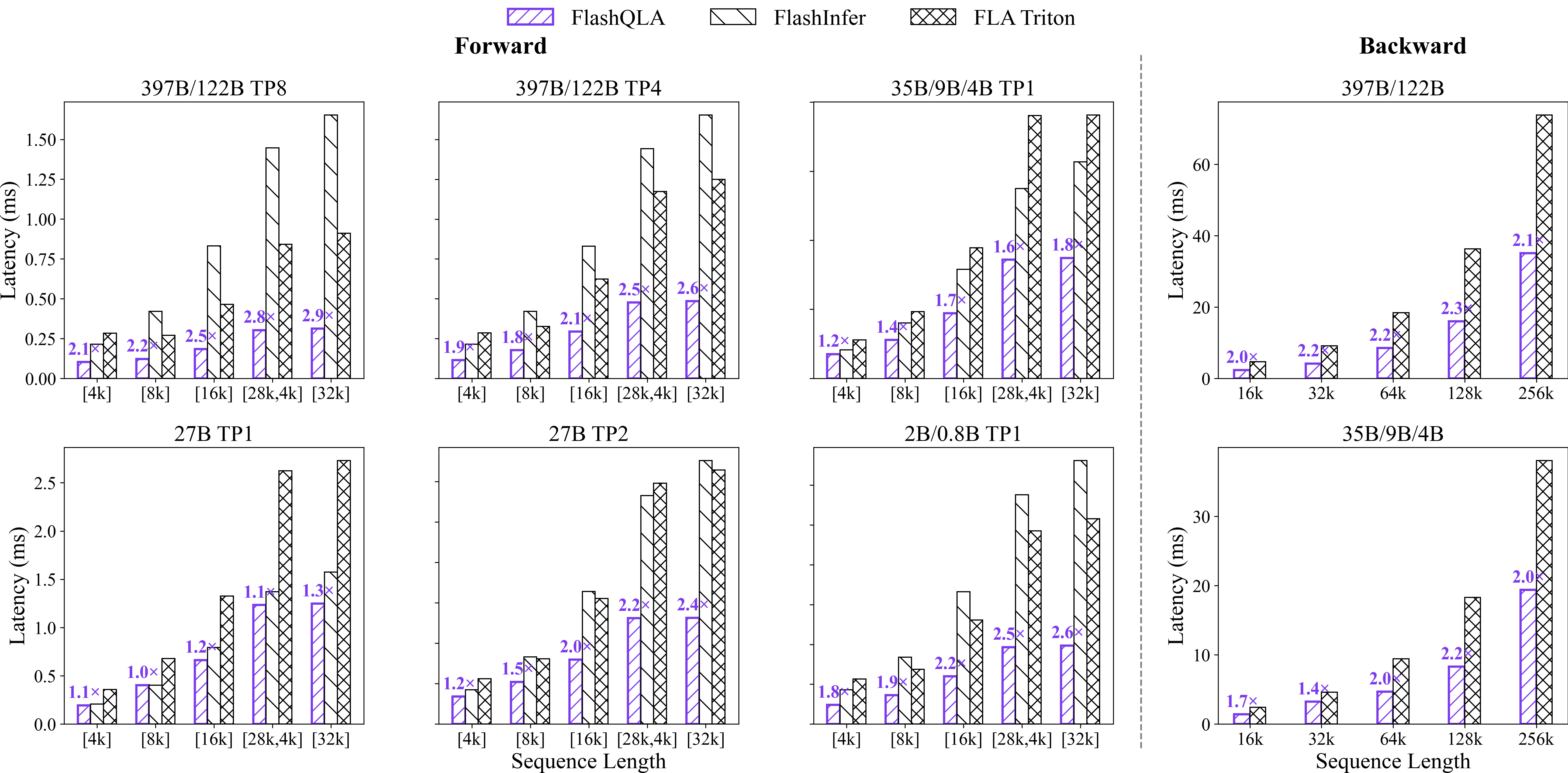
Specifically, the forward (FWD) benchmarks measure single-kernel latency for different models and TP settings under varying batch lengths, while the backward (BWD) benchmarks examine the relationship between total token count within a batch and latency during a single update step.
Selected H200 single-layer forward results:
| Model / TP | Seqlen | $h_{qk}$ | $h_v$ | FlashQLA | FlashInfer | FLA | vs FLA | vs FI |
|---|---|---|---|---|---|---|---|---|
| 397B/122B TP8 | 1x32768 | 2 | 8 | 0.310ms | 1.653ms | 0.913ms | 2.95× | 5.33× |
| 397B/122B TP8 | 1x16384 | 2 | 8 | 0.184ms | 0.833ms | 0.465ms | 2.53× | 4.53× |
| 397B/122B TP8 | 24576+8192 | 2 | 8 | 0.302ms | 1.242ms | 0.767ms | 2.54× | 4.11× |
| 397B/122B TP4 | 1x32768 | 4 | 16 | 0.486ms | 1.654ms | 1.250ms | 2.57× | 3.40× |
| 397B/122B TP4 | 1x16384 | 4 | 16 | 0.292ms | 0.832ms | 0.623ms | 2.13× | 2.85× |
| 27B TP2 | 1x32768 | 8 | 24 | 0.659ms | 1.616ms | 1.564ms | 2.37× | 2.45× |
| 2B/0.8B TP1 | 1x32768 | 16 | 16 | 0.493ms | 1.640ms | 1.285ms | 2.60× | 3.33× |
| Sym h32 | 1x32768 | 32 | 32 | 0.877ms | 1.554ms | 1.952ms | 2.23× | 1.77× |
The speedup grows with TP degree because FlashQLA improves SM utilization via intra-card AutoCP in the exact regimes — TP sharding and small head number — where the baseline leaves SMs idle.
Usage#
FlashQLA exposes both a high-level API matching FLA’s signature and low-level fwd/bwd entry points:
import torch
from qla import chunk_gated_delta_rule

o, final_state = chunk_gated_delta_rule(
    q=q,                            # [B, T, H_q, K]
    k=k,                            # [B, T, H_q, K]
    v=v,                            # [B, T, H_v, V]
    g=g,                            # [B, T, H_v]
    beta=beta,                      # [B, T, H_v]
    scale=scale,
    initial_state=initial_state,    # optional, [B, H_v, K, V]
    output_final_state=True,
    cu_seqlens=cu_seqlens,          # optional, varlen support
)
Requirements: SM90, CUDA 12.8+, PyTorch 2.8+. Install:
git clone https://github.com/QwenLM/FlashQLA.git
cd FlashQLA && pip install -v .
Acknowledgments#
FlashQLA is inspired by Flash Linear Attention, FlashInfer and TileLang. We thank these communities for the reference implementations.
Citation#
If FlashQLA is useful for your research, please cite:
@misc{flashqla2026,
    title  = {FlashQLA: Flash Qwen Linear Attention},
    author = {Zhang, Chengruidong and Lin, Xi and Jiang, Huiqiang and Wang, Zekun and
              Li, Xiao and Cao, Yizhong and Zhuang, Bohan and Men, Rui and Zhang, Jianwei and
              Zheng, Bo and Lin, Junyang and Liu, Dayiheng and Zhou, Jingren},
    year   = {2026},
    publisher = {GitHub},
    howpublished = {\url{https://github.com/QwenLM/FlashQLA}}
}
原文来自 千问 Qwen Team,版权归原作者。
正文采集于 ,内容更新以原文为准。